I don’t have classes on Friday this semester. I spent most of the day doing research (learning how to do exploratory factor analysis  on some survey data).

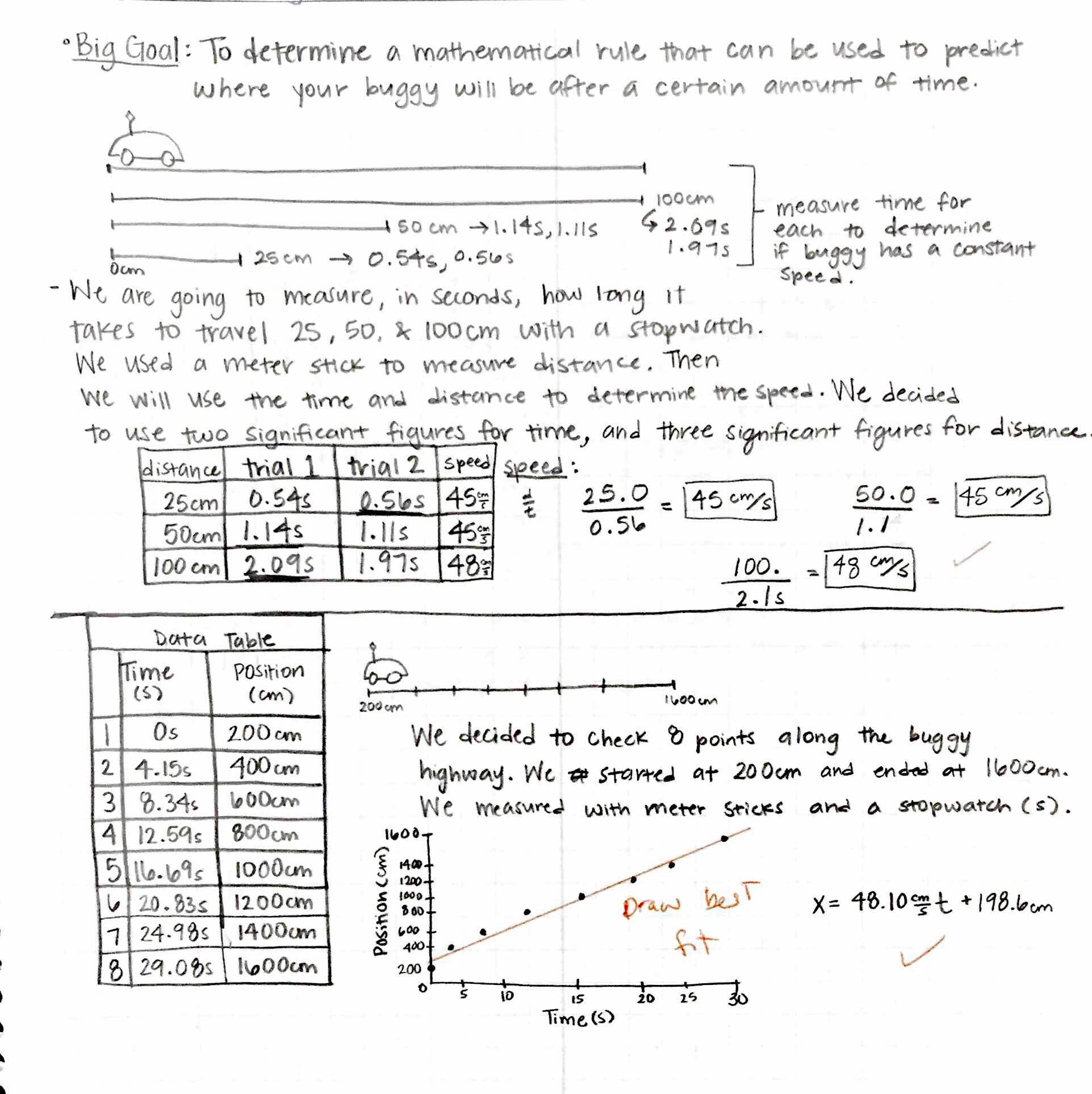
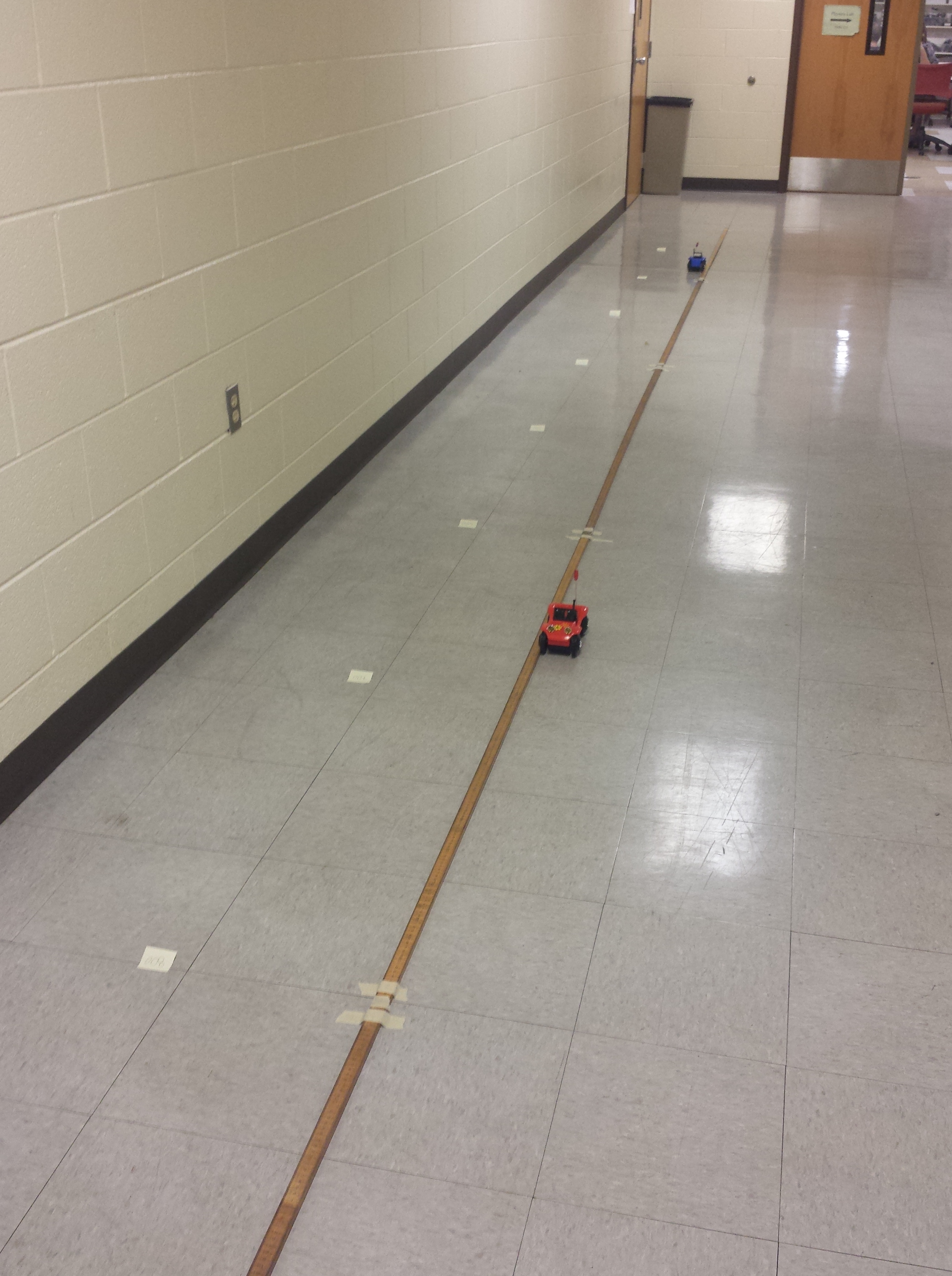
Teaching-wise, I started grading lab books. Here is a photo of one students’ lab book fro the buggy lab to offer a feel for the kind of work they are expected to turn in. Keep in mind, these are lab books (not lab reports).

There are also 4-6  summarizing at the end. This lab had following questions:

1. How can you decide by looking at your position vs. time graph whether or not the buggy moved at (roughly) a constant speed or not?
2. What value for the buggy’s speed did you get using your “quick and easy” method? How did this compare to the slope of the mathematical rule you determined?
3. Write down the mathematical rule you determined for the buggy’s motion.
   1. What would be different if the buggy had moved faster?
   2. What would be different if the buggy had started at a different location?
   3. What would be different if the buggy had moved in the opposite direction?
4. What did you learn today that might help you address the challenge lab?

Most groups were able to make good connections between slope and speed, intercept and initial position, and the sign of the slope with direction. Based on the lab books, one group, however, did struggle to make those connections.

Today, I have spent some of the day prepping for our next meeting. Students will have read over the weekend two sections from the text that will build on the buggy lab: a section on position vs time graphs and a section on uniform motion. We will also return to class next week with some clicker questions to review these ideas.

Then students will revisit motion detectors to make graphs. [Last time we just used them to make motion diagrams.] This lab exploration starts off just qualitative, with students making predictions and observations as well as doing some graph matching; but it transitions to quantitative stuff with students re-applying what they learned about linear fits (in Logger Pro) last week to extract velocity information. The last task of the lab exploration has them re-measure the speed of their buggy using this new technique.

Then we will have our first day of collaborative problem-solving.

The plan for problem-solving is

1.  Staged Problem-solving:  We are following Knight’s break-down for problem-solving into “Prepare, Solve, Assess”. So students will be given a problem, and groups will first be asked just to prepare on whiteboard. Preparing at this point involves making pictures, collecting important information, and doing preliminary calculations. A little bit of discussion to highlight different aspects of students’ work. Before beginning the problem, we will ask students to make guesstimate for, “Best Guess, Definitely too Long”.  Then they will solve the problem. Discussion similar as needed. Then they will be asked to assess in variety of ways, including checking against their guesstimate, making sure they have actually answered the question, checking units.
2. Un-staged Problem-solving:  Students have to do each of the steps, prepare, solve, assess, but we won’t pause to discus between each.

Both problems are two-body uniform motion that don’t involve simultaneous system of equation. For example, one has two cars traveling the same trip, one traveling faster but leaving leaving at an early time. Question is who will finish first and how long will they have to wait for the other to arrive? Students will be required as part of “solve” to make a position vs time graph. Groups who finish solving early will be asked to solve for other aspects, including when and where did they pass each other.

If we have time, I want students to use their skills to solve a real buggy collision problem. Since in the lab exploration, they already got the speed of their buggy again, this may be doable time-wise. I’d like to do this so they can use their skill to actually predict something, but it also rehearses something like our “Challenge Lab”.

Yesterday, in my pilot section of revised algebra-based physics, we talked about uncertainty for a bit and then students did the buggy lab. Lab went well. Only change was groups who finished early had to revise/apply their model to make a prediction and test it out (e.g., buggy starting somewhere new, going in opposite direction, where will it be/ or how long will it take to ___ ).

Here is a picture of the buggy highway we set up in the hallway:

Lab Uncertainties: Last Year vs This Year

For uncertainties, we used to have students estimate measured uncertainties, calculate percentage uncertainties, and then have students identify the largest (average) percentage uncertainty of all their measurement types before using that to propagate uncertainty to any calculated results (e.g., slope).

Now, we have students take multiple or repeated measurements to help inform judgments about which digits seem “trustworthy”. We defined trustworthy digits as those that don’t change much upon repeated measurements. This leaves some room for ambiguity which is fine– for example, we had clicker question to identify where the smallest trustworthy digit was with repeated measurements of 12.69 ft and 12.91ft. Either the ones place or the tenths place could be justified. For propagating uncertainty, we have students use the rules for significant figures, because that’s what is taught in Knight’s College Physics. Overall, I’m pretty happy with this approach. In the first lab, we actually had interesting conversations about uncertainty instead of mind-numbing conversations about how to apply the rules.

For example, one group had measured time repeatedly in their “Quick and Easy” speed calculation (before a more careful investigation), and found that their time measurements really only had 1 sig fig (something like 5.87s, 7.07s, 6.32s). They were unhappy with rounding 24 cm/s down to 20 cm/s. They felt like this was losing accuracy. When they later found the speed using graphical methods, they got 19 cm/s. They were really surprised that their 1 significant figure rounding was closer than their 2 significant figure rounding. One student said that hadn’t realized that such a thing was possible.

Today was the first day in a pilot section of a newly developed algebra-based physics course. I am piloting one section and a colleague is piloting the same in a second section.

Some details about the changes include

Text: Changed from a Home-grown text to Knight’s College Physics

Homework: Changed from no HW to Mastering Physics

Labs: Changed from confirmation labs to a variety of lab format including qualitative explorations of phenomena, guided investigations, and application/challenge labs.

Equipment: From teacher control over lab equipment to open student access to a variety of vernier lab equipment (sensors, cart, tracks, etc).  Each day students must retrieve and return at last some their equipment. On “challenge” labs, students have to decide what equipment they want to address the challenge.

Groups: From lots of unstructured group work to more structured group work (a lot of this came about from students having free access to equipment… we only wanted one person per day to be retrieving/returning equipment). This led us to think more critically about group roles. We still have some work to do in building assessment (peer/self/whatever) to our structure.

Hours:  From Two 2.5 hours studio session + one 1.5 hour lecture to two 3 hour student sessions.  Mini-lectures are interleaved with collaborative problem-solving, labs, clicker questions, etc.

Clickers: Clickers were used exclusively in the 1.5 hour lecture, now they are integrated into the studio sessions.

What are the biggest differences in philosophy?

– Units were organized around “Culminating Challenge Labs” (like practicals in Modeling Instruction).  We designed backwards–asking first what do we want students to understand and be able to do –> then what lab challenges would representatively sample that terrain of understanding –> then finally what learning experiences would give us confidence students would be able to succeed. Our lab activities and problem-solving sessions are intended to equip students with the skills necessary to be successful with the challenge lab. This semester, we’ll be discovering what gaps we’ve made to large and what gaps we’ve overly smoothed over.

– Students having open and free access to the lab equipment is rooted in us trying to give students more agency in the lab. Previously, it always felt like, “we owned the lab equipment” and we set it out for students to use when and how we wanted. We are trying to provide an environment where students feel like it’s their equipment and they get to use it when they need it. Part of that of course is helping them to feel confident in their ability to use it, but releasing control. We will be working on getting the balance right, but I’m happy this is a driving factor of our course.

– A stronger focus on qualitative understanding and conceptual reasoning. We have better balance, which is largely supported by having the new text, using “lab explorations” to introduce topics, and implementing collaborative exercises and clicker questions that focus on that aspect. We tend to move from phenomena –> qualitative representations –> quantitative representations.

Outline of First Day: Introduction and Motion Diagrams

1 hour for course introduction /logistics and pretest

1 hour to interactive lecture demos, clicker questions, and collaborative exercises about motion diagrams

1 hour for lab introduction to logger pro and motion detectors (I created a file to have motion detector make motion diagrams instead of graphs… students practice getting equipment for the first time, connecting their equipment, accessing software, and then they are guided to make predictions/observations for various motions of objects including their hands, fan carts, etc.)

Overall, it went well.