Day 4 Physics II Brain Dump

I. Warm-up Mini Calculation, Clicker Question, and Problem: A quick warm-up to review.

Calculation: Students were given questions to find wavelengths in air of the frequencies at the extreme of human hearing range. They were first asked to state which should be larger and why, and also to give a ballpark estimate for what their guess this distances might be.

Clicker: Students were shown a story graph and a snapshot graph for a wave, both with quantitative information, and asked to determine the wave speed.

Problem: Students were given a problem about a boat on ocean waves. They were given information like wave amplitude, wavelength and wave speed, and they were asked to first construct a snapshot graph and story graph, and then to construct velocity vs. time and acceleration vs time graphs for the boat.

II. Direct Instruction: Showing a PhET Sound Demo, to introduce idea of waves traveling not just in a line but spreading out in 2D and 3D. The simulation makes it easy to link back to story graphs and snap shot graphs. Beyond that, I had two goals here. Point out that the amplitude of the waves seems to go down as it travels away from the source. Our goal today was to build up the tool’s that would help us explain why that happens. My second goal was to introduce the new representation of “wave front” diagrams, linking this idea to their reading about spherical waves –> plane waves.

III. Invention Task: Students were given the following task for an invention task

Screen Shot 2016-02-05 at 1.20.40 PM

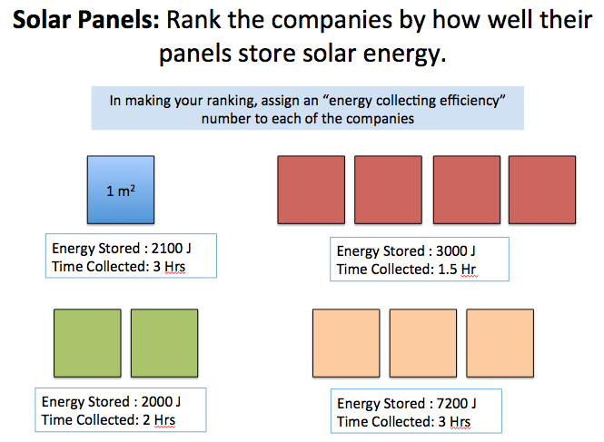
Students caught on to this pretty quick. We had some (rather limited) discussion, which led into direct instruction described below.

IV. Direct Instruction on Intensity, Power, and Energy, plus an Example Problem: I leveraged the invention task to introduce the concepts of Intensity. After briefly introducing the idea, I applied it to a problem about using a lens to focus light (How much energy passes through lens each second; what is the intensity of the light after focusing).

V. Student Problem-Solving: Students were given two problems–one about how much energy an ear drum absorbs at a rock concert; and another problem to estimate how big the largest solar array in america must be.

VI. Direct Instruction and then Clicker Questions to Extend the Intensity Idea:  Had some brief direct instruction and clicker questions to extend the idea of intensity to a sound spreading as a spherical wave (1/r^2). Some of the instruction and questions were meant to pose this as a way of explaining why sound loudness decreases with distance—and to distinguish dampening (energy transforms to thermal) vs energy spreading (same amount of energy becoming less concentrated). After class, a student had lots of questions about this and the 2nd Law of thermodynamics.

VII.  Direct Instruction and Clicker Questions on Decibel Scale: This was brief, mostly to give student an intuitive sense for the decibel scale, rather than a formula sense.

VIII. Problems we didn’t get to: Students were supposed to end the day with a problem applying the idea of intensity decreasing in a spherical wave to calculate how the sound intensity level in dB decreases, but we were tired and running out of time.

Notes: With no lab on the day, it was kind of a slog, but not as bad as some no lab days can be. There lots of opportunities for student to think, discuss, work problems, etc,… but ultimately we needed a little more space in the day for play in order for us not be exhausted. This should be my new design principle–is there enough play?

Day 3 Physics II Brain Dump

This is our first day of waves, after a week of studying oscillations. [Sorry again for the wordy brain dumps, but documenting what I’m doing is just easy to off-load this way].

  1. Warm-up: As they walk in, students are asked to grab a microphone, plug into a Logger Pro, and play around with sounds. The default setting on Logger Pro is about 0.03s of data collection so its a good time scale for seeing things. Students are given some suggestions as what to try such as singing a note like “ahh”, “ooh”, “whistling a note”, “snapping their fingers”… but encouraged to explore. Lastly,  students are asked to find a sound that looks the most sinusoidal and apply the curve fit method to determine the frequency of that sound. I circulate around a fun conversations with students about what they are seeing, ask them what it means that the frequency is 250 hz etc. Students also had lots of interesting questions, too. I ended this exploration with some brief bridging commentary about our transitioning from talking about localized oscillations (e.g., mass on a spring) to waves … by means of asking the question, “How does the oscillation in your vocal chord show up as an oscillation inside the microphone?” and that our study of waves will be about how oscillations (or vibrations) are transmitted from one location to another through a medium.
  2. Direction Instruction with PhET Simulation and a Slinky: I motivate the need to step away from sound waves to spend some time studying waves in a situation that is more concrete and more visible–waves on a string. With the PhET simulation (and later the slinky), I show some wave pulses and talk about the typical transverse wave stuff (each of the objects is moving up/down), even though our eyes track what looks like an an “apparent” motion to the right. Then I orient students to the wave-speed. I repeat a bit of this with the slinky, focusing on each coil is doing, vs what the pulse appears to do.
    • First Clicker Question is what effect making a bigger pulse on the slinky will have on the wave speed. Students vote, discuss, and then we observe. A big idea here is that you while you can control with your hand motion what Amplitude and the Width the Pulse has, you can’t control how fast that pulse moves away from you.
    • I then ask students to think about what if anything we could do to change the wave speed. I then model how increasing the tension changes wave speed. We then use plastic slinky vs a metal slinky to show the effect of mass.
    • Students are introduced to the relationship for wave speed: involving Tension and linear mass density. I don’t say much about linear mass density except to show an equation and say how you would measure it.
    • 2nd Clicker Question: With a piece of string, I go about measuring its linear mass density: I measure it’s length with a meter stick and put in on the scale to find the mass, and calculate its linear mass density. The clicker questions asks students how the linear mass density would change if I cut the string in half. Students did surprisingly well with this… most offered explanation that both numerator and denominator. It’s here that I turned attention to the meaning of linear mass density–
    • 3rd/4th clicker question is just a question about how the wavespeed on a guitar should compare as string thickness goes up and tension is changed using pegs. This was all pretty easy for students after all the demos.
  3. Problem Solving: Students are then asked to put this into problem-solving. Once again, I opt for no sample problem. Just some “must haves” for what must be on a whiteboard. The problem they worked was mostly just an application of the ideas of linear mass density, what factors effect wave speed, but the problem also gave data in which you must infer the wave speed.  Specifically, it gave the length of the string and the time for a pulse to across it (50 ms). More than one groups treated a value of time as 50ms instead as a speed of 50 m/s… Other than that a few groups had difficulty with square-roots and simplifying expressions. Next year I will make the problem a little more challenging by adding extraneous information about the amplitude of the pulse (links back to the demos).
  4. Measuring Speed of Waves:  Going back to the slinky, I ask some questions that lead me into measuring the speed of a pulse on the slinky. The strategy was basically to send a pulse down the slinky and time how long it takes to get to one end, bounce back, and arrive back at me.  This becomes the model for how students will do this for the speed of sound lab. The speed of sound lab I do is pretty much the one published by Vernier in “Physics with Vernier”. Students place microphone on open end up a PVC pipe, and close off the other. Students snap their fingers to create a “sound” pulse. They can observe that finger snap pulse return again and again. They can use that data and reasoning in order to make distance traveled for clock reading plot to get speed of sound: Every group but one got speed between 335 m/s and 345 m/s.
  5. Direct Instruction on Sinusoidal Waves: Back to the PHET Simulation. Mostly here I’m showing that when the source itself undergoes simple harmonic motion, the resulting wave takes a sinusoidal form. This is also a place where wavelength gets introduced, and connection between wave speed, wavelength, and frequency gets introduced.
    • I first take some time to “pause” the simulation and talk about this as a “snap shot” graph (this is language from Knight book, and I like it), really a Amplitude of the Wave vs. Position along the String graph. I talk about how you can in a single “snap shot” graph you can see wavelength (crest to crest) but you can also see wave speed by noting that the location of crests appear to move forward in subsequent snapshots.
    • I then ask students to pretend putting a motion detector underneath one of the green “pieces of string” on the simulation, and talk about what the graph would look like from the motion detector. Using the language from Knight, we call these history (or story) graphs. Each piece just undergoes SHM, what we studied last week. I do some comparison and contrast of Snapshot vs. History graphs as a way to distinguish wavelength from period.
    • Students practice reasoning about these graphs with clicker questions. One clicker Question in particular shows a “snap shot” graph of a sinusoidal wave and you are also told wave velocity is to the right. Students are asked which direction a point on the string is moving–up, down, right, left, not moving. We spent a lot of time discussing this, as it got the heart of understanding lots about waves and these representations. A few other clicker questions lead into introducing the relationship between wavelength, wave speed, and frequency. This could use some tweaking.
    • Finally, a bit of pre lab discussion points out how “easy” it had been for us see wavelength with a string. You take a snapshot and measure crest to crest. Using PhET simulation, I take time to show them something else about wavelength, by focusing attention on the motion of two pieces separated by a wavelength. The two pieces always bob up and down exactly together–whenever one is up, the other is up. So on and so forth. I also point out that at half wavelengths, the pieces of string are always doing the opposite. I introduce the language of “in phase” and “out of phase”, and tell them that we can use the “in phase” and “out of phase” technique to identify the wavelength for waves you can’t see so easily. This leads us into the final lab exploration for the day. I need to add some clicker questions to this, so it’s less me lecturing.
  6. Final Lab Exploration: So, this didn’t quite work out because of some equipment issues (the speakers in the laptops basically can’t play pure tones very well), but the idea was that students were going to use a tone generator to make a pure sound and record data with a microphone. From the data, they would then determine the frequency (using the curve fit method). Then they would predict what the wavelength should be, based on the relationship between wavelength, wave speed, and frequency. Then, they would use the “in phase” method to check their predictions–moving a second microphone to a distance equal to wave length–show that the two oscillations are in phase. Move a second microphone to a distance equal to 1/2 wavelength–show that the two oscillations are out of phase. We ended up doing this very informally, without any lab write up.

Thoughts: One of the things that I’m enjoying about this semester is we are doing a lot of “back-and-forth” between lab work, discussion, and direct instruction. While I am very comfortable managing this, that’s not going to be the case for others in the department. There’s a lot of comfort in putting laboratory stuff at the end of the day… their is a lot of concern about students finishing at different times, etc. I’m curious what advice people have for this. I feel like I’ve learned over time how to manage this (probably not optimally I’m sure), but it’s definitely an area of concern for instructors.

Blog at WordPress.com.

Up ↑